ICU Serum Sodium Prediction
Background:Dysnatremia is a central electrolyte disorder in the intensive care unit (ICU) that results in poor prognosis and increases in-hospital mortality risk. The existing clinical method for estimating serum sodium level is based on the experience of doctors, which is subjective and difficult to predict the patient’s subsequent status. To simplify this difficulty, we aimed to develop an assistance system for doctors to predict short-term serum sodium changes.
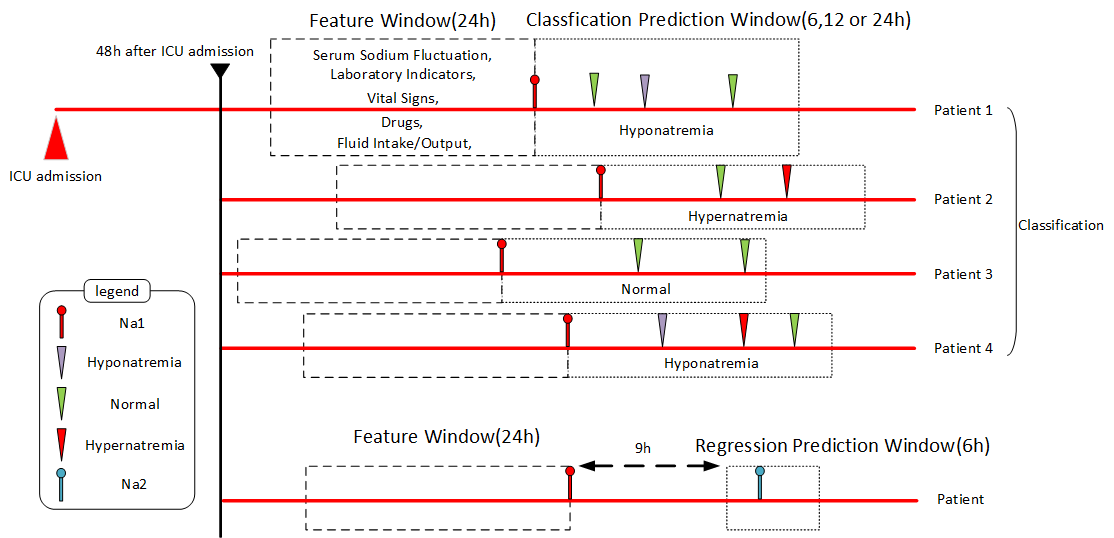
Methods:Patient samples with abundant feature variables were extracted from electronic health records (EHR) using a dynamic sliding window method. The end point of the feature window was the patient’s initial serum sodium record 72 hours after admission, with the starting point set at 24 hours before the end point. Five machine learning classification models were developed based on the patient clinical indicators extracted from the feature window, which were used to predict the subsequent serum sodium status in the prediction window for time intervals of 6, 12, and 24 hours. A regression analysis was performed on the patients’ serum sodium values. The least absolute shrinkage and selection operator regression model was applied for feature selection, and four machine learning models were trained to predict serum sodium values. The prediction results of all models were evaluated and compared, and SHapley Additive exPlanations (SHAP) was utilized to assess the interpretability of the best performing classification and regression model.
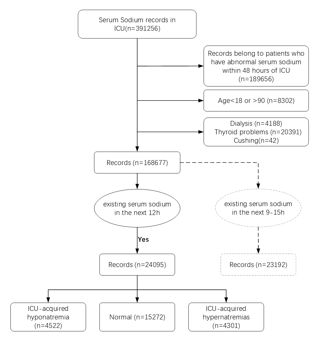
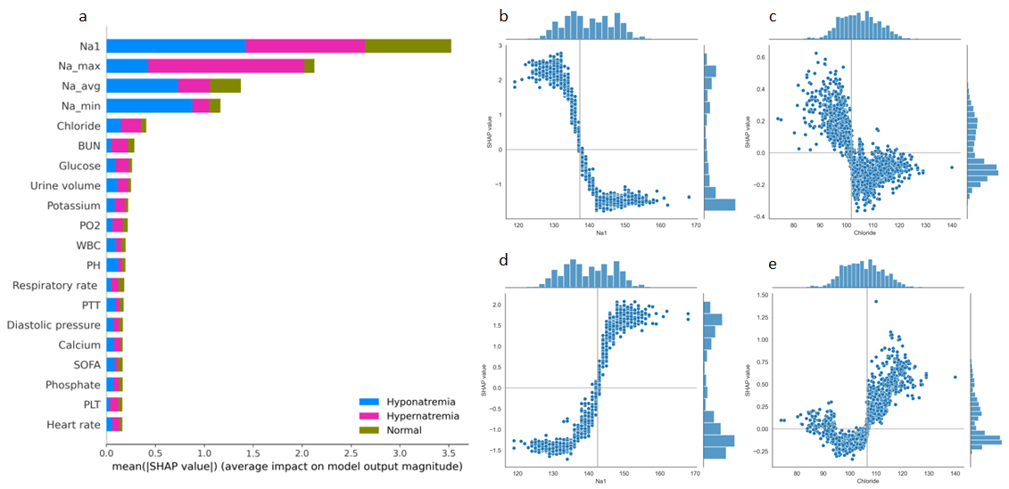
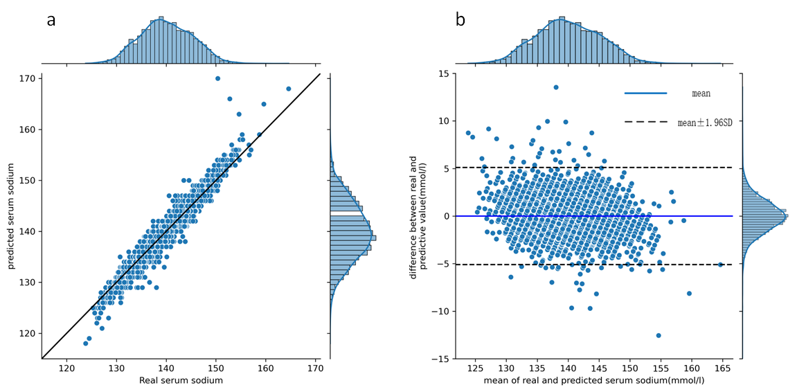
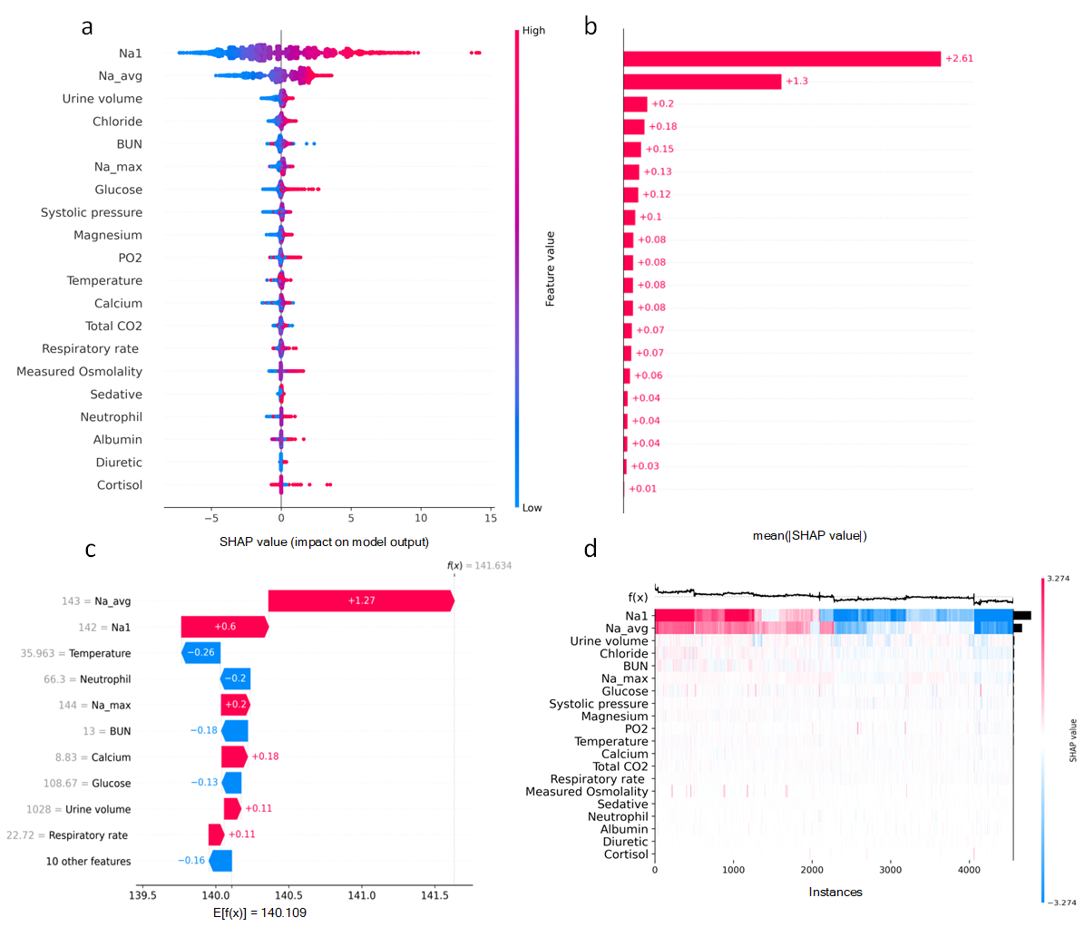
Results:In the 12-hour classification prediction window, there were 4522 hyponatremia samples, 15272 normal serum sodium samples and 4301 hypernatremia samples. Among the classification models, the best model was LightGBM with accuracy, sensitivity, specificity and F1 score of all 0.86. All regression models performed well and the LightGBM model achieved the best results with r-square = 0.86, root mean squared error = 2.55 and mean absolute error = 1.86. Based on the interpretable SHAP analysis of the mentioned models, initial serum sodium, chloride, urine volume, blood urea nitrogen and glucose had essential effects on the patients’ following short-term serum sodium levels.
Conclusions:The proposed methods can accurately predict short-term serum sodium levels in the following 24-hour prediction window. And our methods can reasonably explain and visualization the prediction results utilizing clinical indicators.
